Working with data
This page shows how to use pypalmsens to interface with your measurement data.
The pypalmsens.data submodule contains wrappers for the PyPalmSens .NET SDK libraries.
These are the same libraries that power the PSTrace software.
Measurement
>>> measurements = pypalmsens.load_session_file('Demo CV DPV EIS IS-C electrode.pssession')
>>> measurements
[Measurement(title=Differential Pulse Voltammetry, timestamp=12-Jul-17 14:28:58, device=PalmSens4),
 Measurement(title=Cyclic Voltammetry [1], timestamp=12-Jul-17 14:33:10, device=PalmSens4),
 Measurement(title=Impedance Spectroscopy [2], timestamp=12-Jul-17 14:48:42, device=PalmSens4)]
A .pssession file always contains a list of measurements, so we pick the first (DPV) one:
>>> measurement = measurements[0]From there we can query the device info:
>>> measurement.device
DeviceInfo(type='PalmSens4', firmware='', serial='PS4A16A000003', id=9)
As well as other measurement metadata:
>>> measurement.title
'Differential Pulse Voltammetry'
>>> measurement.timestamp
'12-Jul-17 14:28:58'
>>> measurement.channel (1)
-1| 1 | For multichannel measurements |
There are two ways to access the data.
m.dataset returns the raw data that were measured, analogous to the Data tab in PSTrace.
m.curves returns a list of Curve objects, which represent the plots.
For more information, see the Measurement reference.
Curve
A measurement can contain multiple curves, this measurement has only 1 with 219 data points:
>>> curves = measurement.curves
>>> curves
[Curve(title=Curve, n_points=219)]
>>> curve = curves[0]
From here we can query some Curve metadata:
>>> curve.title
Curve
>>> len(curve)
219
>>> curve.x_label, curve.x_unit
('Potential', 'V')
>>> curve.y_label, curve.y_unit
('Current', 'µA')
Use the .plot() method to show a simple plot of the data.
This depends on matplotlib being available.
>>> fig = curve.plot() (1)
>>> fig.show()| 1 | This returns a matplotlib Figure. |
This results in this plot:
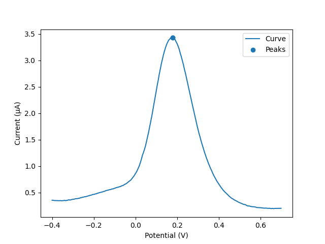
The data has a single peak stored in the measurement. We can retrieve it using:
>>> curve.peaks
>>> peaks
[Peak(x=0.179102 V, y=3.42442 µA, y_offset=0.26371 µA, area=0.818265 VµA, width=0.221563 V)]
To find the peak ourselves, use .find_peaks():
>>> peaks = curve.find_peaks()
>>> peaks
[Peak(x=0.179102 V, y=3.42442 µA, y_offset=0.26371 µA, area=0.818265 VµA, width=0.221563 V)]
An alternative method for CV and LSV is available under curve.find_peaks_semiderivative().
For more info on this algorithm, see this Wikipedia page.
|
Peak finding
Depending on your data, the peak finder may not always find peaks on the first try.
Sometimes the parameters need to be tuned, see |
You can do filtering using .smooth(). Note that this updates the curve in-place.
>>> curve.smooth(smooth_level=1)Or alternatively using a Savitsky-Golay filter:
>>> curve.savitsky_golay(window_size=3)To make your own plot or run your own data processing or analytics script,
the raw x and y data can be accessed through curve.x_array and curve.y_array.
These both return DataArray objects, which can be converted to floats or numpy arrays.
>>> curve.x_array
DataArray(name=potential, unit=V, n_points=219)
>>> list(curve.x_array)  (1)
[-0.399962, -0.394962, ..., 0.692698, 0.697776]

>>> curve.y_array
DataArray(name=current, unit=µA, n_points=219)
>>> np.array(curve.y_array)  (2)
array([0.352146, 0.351192, ..., 0.19908 , 0.199557])| 1 | Convert to list… |
| 2 | …or numpy array |
For more information, see the Curve reference.
Peak
The peaks is a small dataclass containing peak propersies.
Stored peaks can be retrieved from a Curve (e.g. if PSTrace stored peaks in the `.pssession file).
>>> peaks = curve.peaks
>>> peaks
[Peak(x=0.179102 V, y=3.42442 µA, y_offset=0.26371 µA, area=0.818265 VµA, width=0.221563 V)]
Many peak properties are accessible from this object.
>>> peak.x, peak.y
(0.179102, 3.42442)
>>> peak.width
0.2215
>>> peak.area
0.8182
>>> peak.left_x, peak.right_x
(-0.35465, 0.647385)
>>> peak.value (1)
3.1607| 1 | The peak value is the height of the peak relative to the baseline |
For more information, see the Peak reference.
DataSet
The raw data are stored in a dataset. The dataset contains all the raw data, including the data for the curves.
>>> dataset = measurement.dataset
>>> dataset
DataSet(['Time', 'Potential', 'Current'])
A dataset is a mapping, so it acts like a Python dictionary:
>>> dataset['Time']
DataArray(name=time, unit=s, n_points=219)
>>> dataset['Potential']
DataArray(name=potential, unit=V, n_points=219)
To list all arrays:
>>> dataset.arrays()
[DataArray(name=time, unit=s, n_points=219),
 DataArray(name=potential, unit=V, n_points=219),
 DataArray(name=current, unit=µA, n_points=219)]
Some commonly used arrays can be retrieved through a method:
>>> dataset.current_arrays()
[DataArray(name=current, unit=µA, n_points=219)]
>>> dataset.potential_arrays()
[DataArray(name=potential, unit=V, n_points=219)]
Datasets can be quite large and contain many arrays. Therefore, arrays can be selected by name…
>>> dataset.array_names
{'current', 'potential', 'time'}
>>> dataset.arrays_by_name('time')
[DataArray(name=time, unit=s, n_points=219)]…quantity…
>>> dataset.array_quantities
{'Current', 'Potential', 'Time'}
>>> dataset.arrays_by_quantity('Potential')
[DataArray(name=potential, unit=V, n_points=219)]…or type:
>>> dataset.array_types
{<ArrayType.Current: 2>, <ArrayType.Potential: 1>, <ArrayType.Time: 0>}
>>> dataset.arrays_by_type(pypalmsens.data.ArrayType.Current)
[DataArray(name=current, unit=µA, n_points=219)]
Note that for larger datasets these methods can return multiple DataArrays. Data from a Cyclic Voltammetry measurement can contain multiple scans and can therefore the dataset can contain multiple arrays per array type.
>>> df = dataset.to_dataframe()
>>> df
     Time Potential   Current     CR ReadingStatus
0     0.0 -0.399962  0.352146  10 uA            OK
1     0.2 -0.394962  0.351192  10 uA            OK
2     0.4 -0.389884    0.3469  10 uA            OK
..    ...       ...       ...    ...           ...
216  43.2  0.687698  0.198544  10 uA            OK
217  43.4  0.692698   0.19908  10 uA            OK
218  43.6  0.697776  0.199557  10 uA            OK

[219 rows x 5 columns]
Any new Curve can be generated by passing the x and y keys to use:
>>> list(dataset)
['Time', 'Potential', 'Current']  (1)
>>> curve = dataset.curve(x='Time', y='Potential', title='My curve')
>>> curve
Curve(title=My curve, n_points=219)| 1 | Any combination of these will work |
For more information, see the DataSet reference.
DataArray
Data arrays store a list of values, essentially representing a column in the PSTrace Data tab.
Let’s grab the first current array:
>>> array = dataset.current_arrays()[0]
>>> array
DataArray(name=current, unit=µA, n_points=219)
An array stores some data about itself:
>>> array.name
'current'
>>> array.type
<ArrayType.Current: 2>
>>> array.unit
'µA'
>>> array.quantity
'Current'
Arrays act and behave like a Python Sequence (e.g. a list).
>>> len(array)
219
>>> min(array)
0.193358
>>> max(array)
3.42442
>>> array[0]
0.352146
Arrays support complex slicing, but note that this returns a list.
>>> array[:5]
[0.352146, 0.351192, 0.3469, 0.345947, 0.344516]
>>> array[-5:]
[0.197411, 0.198127, 0.198544, 0.19908, 0.199557]
>>> array[::-1]  (1)
[0.199557, 0.19908, ..., 0.351192, 0.352146]| 1 | reverse list |
Arrays can be converted to lists or numpy arrays:
>>> list(array)
[0.352146, 0.351192, ..., 0.19908, 0.199557]
>>> np.array(array)
array([0.352146, 0.351192, ..., 0.19908 , 0.199557])
For more information, see the DataArray reference.
EISData
We can retrieve EIS data from an EIS measurement.
Note that the EIS measurement can be multichannel, so .eisdata returns a list.
If you don’t use a multiplexer, we can pick the first (and only) item from the list.
>>> eis_measurement = measurements[2]
>>> eis_measurement
Measurement(title=Impedance Spectroscopy [2], timestamp=12-Jul-17 14:48:42, device=PalmSens4)
>>> eis_measurement.eis_data  (1)
[EISData(title=FixedPotential at 71 freqs [2], n_points=71, n_frequencies=71)]
>>> eis_data = eis_measurement.eis_data[0] (2)| 1 | .eis_data returns a list |
| 2 | Pick the first and only item |
The EISData object can be queried for metadata:
>>> eis.title
'FixedPotential at 71 freqs [2]'
>>> eis.scan_type
'Fixed'
>>> eis.frequency_type
'Scan'
>>> eis.n_points
5
>>> eis.n_frequencies
5
If previously fitted a circuit model in PSTrace, we can retrieve the CDC values:
>>> eis_data.cdc
'R([RT]Q)'
>>> eis_data.cdc_values
[132.146, 11009.9, 3710.55, 3.77887, 0.971414, 6.23791e-07, 0.961612]
And use these to fit a circuit model:
>>> model = pypalmsens.fitting.CircuitModel(cdc=eis_data.cdc)
>>> result = model.fit(eis_data, parameters=eis_data.cdc_values)
>>> result
FitResult(
    cdc='R([RT]Q)',
    parameters=[132.14, 11009.96, 3710.50, 3.78, 0.97, 6.23e-07, 0.96],
    error=[1.51, 4.60, 37.55, 165.04, 25.81, 7.22, 0.94],
    chisq=0.0054,
    n_iter=5,
    exit_code='MinimumDeltaErrorTerm',
)
The raw data can be accessed via .dataset. This results in a DataSet object.
>>> eis_data.dataset
DataSet(['Current', 'Potential', 'Time', 'Frequency', 'ZRe', 'ZIm', 'Z', 'Phase', 'Iac', 'Unspecified_1', 'Unspecified_2', 'Unspecified_3', 'Unspecified_4', 'YRe', 'YIm', 'Y', 'Cs', 'CsRe', 'CsIm'])
Likewise, we can retrieve all the arrays:
>>> eis_data.arrays()
[DataArray(name=Idc, unit=µA, n_points=71),
 DataArray(name=potential, unit=V, n_points=71),
 DataArray(name=time, unit=s, n_points=71),
 ...
 DataArray(name=Capacitance, unit=F, n_points=71),
 DataArray(name=Capacitance', unit=F, n_points=71),
 DataArray(name=Capacitance'', unit=F, n_points=71)]
Subscans
If an EIS dataset has subscans, this is shown in the repr:
>>> eis
EISData(title=CH 3: E dc scan at 5 freqs, n_points=20, n_frequencies=5, n_subscans=4)
>>> eis.has_subscans
True
>>> eis.n_subscans
4
Subscans can be accessed via the .subscans() method.
>>> eis.subscans
[EISData(title=E=0.000 V, n_points=5, n_frequencies=5),
 EISData(title=E=0.200 V, n_points=5, n_frequencies=5),
 EISData(title=E=0.400 V, n_points=5, n_frequencies=5),
 EISData(title=E=0.600 V, n_points=5, n_frequencies=5)]
The subscans are themselves EISData objects.
For more information, see the EISData reference.